Research Areas and Projects
Speech Synthesis Using HMM and Unit Selection
The Hidden Markov Model (HMM)
Speech Synthesis with HMM
Speech Synthesis with Unit Selection
The Hybrid System
Key References and Links
Speech Synthesis Using Hidden Markov Model and Unit Selection
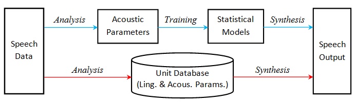
Although the two currently dominant speech synthesis approaches, the hidden Markov Model and unit selection, are both based on raw speech data, they use data in quite different ways. The former approach tries to construct statistical models of various acoustic parameters out of the raw data and generate new speech on the basis of the models. So what's important is not just the statistical models, but also the acoustic model. What parameters to use, how to extract those parameters from real speech and how to construct new speech from those parameters stand at the center of the acoustic model. In contrast, the latter approach follows a different analysis-synthesis path. The speech data are first broken into units, usually phones, and put into a database. In generating new speech the appropriate units are selected from the database and concatenated together. The approriateness of the selection is guided by unit similarity and concatenation smoothness on the basis of linguistic and acoustic parameters (features/contexts). The following diagram depicts the conceptual difference between the two approaches. The path of the hidden Markov model approach is colored blue and that of the unit selection approach red.
The Hidden Markov Model (HMM)
Modelling is a basic scientific method, ranging from the model of an atom to the model of an economy. The basic tension in modelling is that between approximity and manageability. Every model is a representation of reality, but not reality itself. However we want our model to approximate reality. If it's too far off, it doesn't make much sense. On the other hand, the model has to be manageable. If it's too complicated, it's also useless. Therefore, simplification is inevitable in every model. The reason why the hidden Markov model has been successfully adopted in a variety of fields is that it makes a nice trade-off between approximity and manageability.
The hidden Markov model concerns a time series, which covers a wide range of phenomena, including human speech. A time series, basically a process, could be as complex as one can imagine. The model makes things manageable with a bunch of simplifications:
- Finite state set The states in the time series are from a finite set.
- Markov chain The transition to the next state is only determined by the current state. In other words, all the history is contained and represented in the present.
- Stationary transition The transition between states is constant in time.
- State-based observation The observation is determined only by the state at a particular point in time. It has nothing to do with history or other states.
With the above assumptions the hidden Markov model λ consists of the following elements:
-
Initial state probability Π: πi, 1< i <N,
Transition probability A: aij, 1< i, j <N &
Observation probability B: bi(o), 1< i <N,
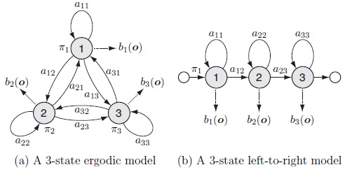
where N is the size of the state set. bi(o) is usually modelled by a mixture of multivariate Gaussian distributions. The following examples are taken from Yamagishi's An Introduction to HMM-Based Speech Synthesis. Apparently (b) is simpler than (a). When we choose (b) instead of (a), we make yet another simplification.
In practical situations the model is hidden from us. What we have are observations. So a useful problem to solve is to figure out the model behind the phenomena. A straightforward principle is the maximum likelihood (ML) criterion: Given the observation sequence O = (o1, o2,..., oT) we want to find the optimal model λ* which maximizes the likelihood of O:
| λ* = | argmax | P | (O | λ). |
| λ |
Once we pick the number of states N, determining the model boils down to calculating the various probability values in the model. There is no direct way to do that. Fortunately a method to approach the values iteratively has been discovered. This is the Baum-Welch algorithm. And it's behind the training process of HMM.
Speech Synthesis with HMM
HMM-based speech synthesis (HTS) is a data-driven approach. The speech data are first analysed into a set of acoustic parameters. Then statistical models of those parameters are trained out of the data. And finally, given a target text, the corresponding parameters are generated out of the models and are used to generate the target speech in turn.
Choice of acoustic parameters
Choosing the correct parameters is the central part of the acoustic model. A good set of parameters should be able to capture essential aspects of human speech, so that when a piece of speech goes through the analysis-synthesis process it still sounds close to the original. The acoustic parameters that are often used in the current HTS systems are spectrum and F0. Different models may be chosen for the spectrum in turn, such as LSP (Linear Spectral Pair) and MFCC (Mel-Frequency Cepstral Coefficients). When a speech wave form is analysed it's segmented into small frames (usually 5ms wide) and the spectral parameters and F0 are computed for each frame within a covering window. After that we have a series of parameter values for each piece of speech data.
Parameter modelling or model training
Parameter modelling here means to build an HMM for a parameter through training with the speech data. In order to achieve smooth target speech the acoustic parameters of a frame are not modelled separately, but with those of surrounding frames. The latter is represented in the velocity and acceleration components. A single Gaussian distribution is enough for the observation probability in the HMM for the spectral parameters. But since F0 is non-continuous (0 for unvoiced parts) a multi-space distribution is needed. An important factor in speech synthesis with the HMMs of the acoustic parameters is the duration of the states. That tells us how many frames each state should occupy in the target speech. It's difficult to derive the state duration from the state transition probability of the acoustic HMM. Hence a duration model needs to be trained separately.
All the acoustic parameters could be trained together. A typical acoustic HMM has the following structure:
-
State 1 (the initial state)
State 2
-
Stream 1 (Mx3 means & variances, spectral parameters static, velocity & acceleration)
Stream 2 (log F0 static)
-
Mixture 1 (weight; mean & variance)
Mixture 2 (weight; mean & variance)
-
Mixture 1 (weight; mean & variance)
Mixture 2 (weight; mean & variance)
-
Mixture 1 (weight; mean & variance)
Mixture 2 (weight; mean & variance)
...
State 4
.
.
State N-1
...
State N (the final state)
Transition Probability (NxN double)
where M is the dimension of the spectral parameters and N the number of states.
HMMs are essentially generalization of the parameters on the basis of speech data. The speech data normally come in sentences. If we treat each sentence as a unit we would build a super model for all the sentences. The generalization in this case would be too difficult to reach, due to the huge diversity. So we need to divide the data space. An obvious improvement is to treat each phone as a unit and build a model for each phone in the phone set. But the phone models of this kind are still too general, well beyond the power of a simply structured HMM. Therefore further division is necessary. The solution is to assign phones from the speech data to various clusters according to their linguistic features/contexts. This is done with a decision tree based on a set of questions related to the linguistic features/contexts. Then an HMM is built for each cluster. The basic assumption behind clustering is that items assigned to the same cluster are similar in terms of the relevant parameters, acoustic parameters in this case.
The structure of an HMM looks very simple. At first glance we would wonder how such a simple model can capture all the complexity of human speech. Now we see the magic of HMM relies heavily on other theories. The acoustic model is one. And the clustering effectively divides a complex problem and assigns a much easier job to HMM. A clear picture of the context of HMM can help us take full advantage of it.
Parameter generation
Now we have all the models for the clustered phones and are ready to synthesize a new speech, given the target text. First the text will be analysed into phones with their linguistic features/contexts. With this information the corresponding clusters in the decision tree can be found. The acoustic parameters corresponding to each target phone will be generated out of the associated HMMs.
Basically this is the reverse process of model training. But the basic principle is the same, that is, the maximum likelihood criterion. In model training we want to find the optimal model that maximizes the likelihood of the observation. Reversely, in parameter generation we want to find the most likely observation O* given the model λ and the pre-determined observation duration T, on the basis of the duration model:
| O* = | argmax | P | (O | λ, T) |
| O |
Using the most likely state sequence q* (instead of all state sequences) to approximate the above value, the problem is divided into the following two:
| q* = | argmax | P | (q | λ, T) & |
| q |
| O* = | argmax | P | (O | q*, λ, T). |
| O |
These equations are much easier to solve. And finally with the sequence of generated acoustic parameter values the target speech can be created with a certain wave synthesizer.
Speech Synthesis with Unit Selection
Speech synthesis with unit selection (TTS-US) is quite a different approach than HTS. It segments speech data into units and synthesizes the target speech by selecting the appropriate units and concatenating them together.
Choice of unit
The unit could be set on different acoustic/linguistic levels, from frames through phones to phrases. And the units used in the same system don't have to be uniform.
Criteria of unit selection
Hunt and Black's pioneering paper proposed a cost function for the unit selection. The cost function consisted of two parts: the target cost for each candidate unit and the concatenation cost for two adjacent candidate units. Thus the principle of unit selection was to choose the units with the minimum total cost for the whole target sentence. This set the framework for later speech synthesis systems adopting the unit selection approach. Generally speaking the first part favours candidates that are similar to the target units and the second part favours candidates that concatenate well with each other.
The similarity between the candidate and target units can be defined in terms of a set of linguistic parameters. When the speech data are processed these parameters can be computed and stored together with the units in the database. And those for the target unit can be computed from the target text. Besides linguistic parameters acoustic parameters may also be used in calculating the concatenation cost, because this relates to two candidate units. The cost function contains a bunch of weights, which reflect the relative importance of various parameters.
Selection algorithm
Given a target text containing n units, and suppose the number of candidates for each unit is in the size of m, the possible combinations of candidate text are approximately mn. Obviously it's not feasible to traverse all the possible combinations to find the optimal one. Some kind of pruning is necessary. A solution is to pick a certain number of best candidates at each step as we construct the optimal target speech unit by unit. This is the widely used Viterbi algorithm with greedy pruning.
Unit concatenation
Since concatenation is part of the unit selection criterion, no complex technique is needed for the final concatenation. But directly putting the selected units together would be too crude. So usually a simple technique such as cross-fade is used in unit concatenation.
The Hybrid System
Now we can compare the above two approaches (HTS and TTS-US) in terms of practicality and effectiveness. Their essential difference may be summarized as this: whereas HTS makes generalization about the speech data, TTS-US uses the data directly. So the quality of TTS-US relies on the quantity and diversity of the speech data. In contrast, with generalization HTS could live with a small amount of data. On the other hand, model training in HTS takes extra time, which is the price of generalization. And more importantly acoustic analysis and synthesis are much more artificial than simple unit segmentation and concatenation. That's why TTS-US generates more natural speech than HTS, given sufficient speech data. If we flip the coin again, this artificiality just gives HTS more flexibility. On the basis of the generated acoustic parameters we could do all kinds of transformation. But the effect of the same transformation with selected units is not as good.
we can list the above comparison in the following table:
| HTS | TTS-US | |
|---|---|---|
| Quantity and Diversity of Speech Data | lower reliance | higher reliance |
| Modelling | necessary | unnecessary |
| Naturalness | lower | higher |
| Flexibility | good | poor |
In the table we see advantages and disadvantages on both sides. A natural question arises: can we combine the two approaches to have the advantages and overcome the disadvantages? The answer is, why not. That's the basic motivation behind the hybrid system, which combines the two approaches in the same TTS system. However, the existing hybrid systems are mostly focused on using HMM to facilitate or further guide unit selection. An example of the former is to use the Kullback-Leibler divergence (KLD) between the models to pre-select units. An example of the latter is to use probability based on the models as the cost function for unit selection.
As a subject of future exploration we might want to mix the two approaches further, so that we could have both naturalness and flexibility. Some specific hybrid approaches toward this direction deserve more experiments.
Key References and Links
References
- P. Taylor, Text-to-Speech Synthesis, Cambridge University Press, 2009 -- A comprehensive introduction to TTS, including the mathematical foundation, linguistics, acoustics, signal processing, historical and current approaches and other aspects.
- A. Hunt & A. Black, "Unit Selection in a Concatenative Speech Synthesis System Using a Large Speech Database," Proc. ICASSP, pp. 373-376, May 1996 -- The pioneering paper of unit selection.
- L. Welch, "Hidden Markov Models and the Baum-Welch Algorithm" -- The author has a clearer explanation. All the hidden assumptions are revealed, which makes it easier to understand.
- The HTK Book -- Everything about the Hidden Markov Model Toolkit.
- J. Yamagishi, "An Introduction to HMM-Based Speech Synthesis" -- A nice introduction to HTS.
- H. Zen, K. Tokuda & A. Black, "Statistical Parametric Speech Synthesis," Speech Communication, vol. 51, pp. 1039-1064, Nov. 2009 -- A comprehensive summary of the unit selection, HMM and hybrid approaches.
- A. Black, H. Zen & K. Tokuda, "Statistical Parametric Speech Synthesis," Proc. ICASSP, vol. 4, pp. 1229-1232, 2007 -- A light weight version of the previous.
Links